Dynamic SIMS: Working with
Cameca Data
Depth
profile data from Cameca IMS-6f SIMS instruments can be exported via ASCII
formatted files. These files, when written to disk, are assigned a file
extension of .dp_ascii and, if exported from the raw
data, include experimental parameters plus two columns of X/Y pairs
representing the etch-time per cycle and the secondary ion intensity in counts
per second (Figure 1). CasaXPS will convert these .dp_ascii
files only when the raw data is exported. Conversion is performed using the Convert option on the File menu or via the toolbar button![]() .
A File dialog window is invoked by these options, in which the .dp_ascii file containing the raw data is selected and the Open button pressed. A new VAMAS file
will be written to the same directory containing the original ASCII data after
which the profile will appear in a new Experiment Frame in CasaXPS. When more
than one profile is of interest, the data can be combined into a single
Experiment Frame via the Convert and
Merge option on the File menu.
Again a File dialog window appears, in which each .dp_ascii
file within the current directory can be selected using the mouse and the Ctrl
key; on pressing the Open button on
the dialog window the entire set of selected dp_ascii
files are converted to VAMAS files and the resulting files loaded into a single
Experiment Frame. The directory containing the original dp_ascii
files will also contain corresponding VAMAS files. Since the conversion process
involves writing new VAMAS files, it is important that the directory containing
the data must have write permission and there is sufficient space on the disk
to receive the new VAMAS file.
.
A File dialog window is invoked by these options, in which the .dp_ascii file containing the raw data is selected and the Open button pressed. A new VAMAS file
will be written to the same directory containing the original ASCII data after
which the profile will appear in a new Experiment Frame in CasaXPS. When more
than one profile is of interest, the data can be combined into a single
Experiment Frame via the Convert and
Merge option on the File menu.
Again a File dialog window appears, in which each .dp_ascii
file within the current directory can be selected using the mouse and the Ctrl
key; on pressing the Open button on
the dialog window the entire set of selected dp_ascii
files are converted to VAMAS files and the resulting files loaded into a single
Experiment Frame. The directory containing the original dp_ascii
files will also contain corresponding VAMAS files. Since the conversion process
involves writing new VAMAS files, it is important that the directory containing
the data must have write permission and there is sufficient space on the disk
to receive the new VAMAS file.
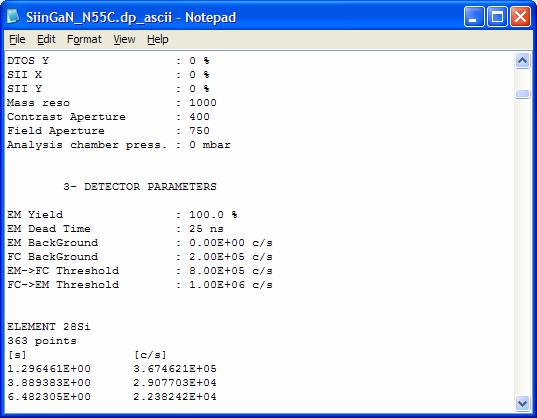
Figure 1: Cameca IMS-6f ASCII formatted data file.
After
conversion to VAMAS format, both the timing information and the intensity units
are adjusted to those used internally by CasaXPS. Most notably, the intensity
unit in the .dp_ascii file is counts per second,
however the intensity in the VAMAS file will be measured in counts per cycle
and the abscissa becomes cycle index. All the associated timing information is
also save with these abscissa and ordinates so that the calibration to depth
and atomic density can be computed later.
Mass
channels used to measure the secondary ion intensity are labelled within the .dp_ascii file using the nominal mass and the element name
abbreviation. When entered into the VAMAS file, the block identifier is
assigned the original string used to label the mass channel, however CasaXPS
attempts to extract the nominal mass and the element abbreviation for use in the
element and transition fields used by the VAMAS format. The concatenation of
these element and transition fields provides the information used to align the
VAMAS blocks within the Experiment Frame and is also used to determine the
isotopic abundance ratio, which in turn is used to determine elemental from
isotopic relative sensitivity factors. If the element/transition fields for a
profile are not correctly assigned, should the user request elemental
sensitivity factors an error message will result. In the event that the element
and transition fields do not contain the element and isotopic information
required to determine the relative abundance for an isotope, then these fields
must be edited to reflect the true isotope used to measure the profile. To edit
these fields:
- Select the VAMAS block(s) in
the right-hand-side of the Experiment Frame.
- Press the
 toolbar button and enter, on the
resulting dialog window, the correct element abbreviation and nominal mass
for the isotope of those VAMAS blocks in the selection.
toolbar button and enter, on the
resulting dialog window, the correct element abbreviation and nominal mass
for the isotope of those VAMAS blocks in the selection.
When the
information on the dialog window is accepted, the VAMAS blocks in the
right-hand-side of the Experiment Frame will be re-organised to reflect the new
assignment.
One way to
check the possible values for the element/transition entries is to use the
Exact Mass Calculator on the Element Library dialog window. Enter a string such
as “Si28” into the text-edit field on the Exact Mass property page and press
the Add Formula button. If a valid isotope string has been entered, then the
string will be entered into the scrolled list above the text-field. Otherwise,
an error dialog will indicated an error occurred. If elemental RSF values are
desired, it is important the string above the VAMAS block in the Experiment
Frame is accepted by the Exact Mass calculator, because this means the database
includes the information necessary for the conversion of the RSF.
Computing the RSF for Si
Data in Figure 1 and Figure 2
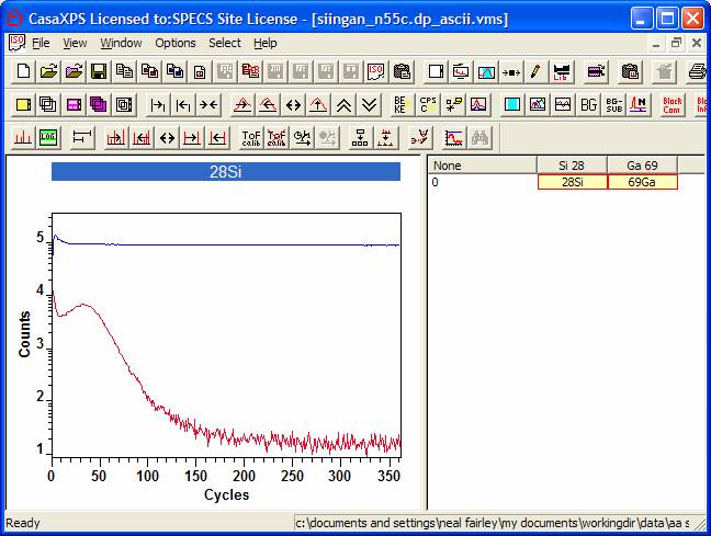
Figure 2: Initial state of the data following conversion to VAMAS format and displayed in CasaXPS.
The
following steps lead to calibrated depth and intensity scales for the data in
the original .dp_ascii file.
- Convert the .dp_ascii file using the Convert option on the File
menu.
- Display the 69Ga data in the
Active Display Tile and left-click on the Active Tile to enable the
toolbar buttons.
- Invoke the Dynamic SIMS Calibration
dialog window by pressing the Dynamic SIMS toolbar button
 .
The top left-most text-field displays the Block Id for the data which is
the current focus of the Dynamic SIMS dialog window.
.
The top left-most text-field displays the Block Id for the data which is
the current focus of the Dynamic SIMS dialog window. - Press the Define Matrix
button on Dynamic SIMS dialog window (Figure 3). Provided no cycles are
selected in the scrolled list below the Define Matrix
button, a dialog window will inform the user that no selection is active
and ask whether all cycles should be updated with the profile in the
Active Tile. Press the Yes
button and observe that the Matrix
Index column of the scrolled
list is updated with the string 69Ga. If any cycle selection has been made
within the scrolled list, then all cycles must be selected before pressing
the Define Matrix button is pressed.
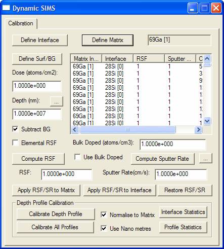
Figure 3
The second
column in the scrolled list is labelled Interface.
For this particular profile, the same matrix is present throughout the etch
cycles and therefore the use of the Interface column is unnecessary. If the
material were a multilayer sample, where RSF and sputter-rates varied between
layers, then the Interface column would need to be populated with strings
corresponding to the different materials characterising the layer structure.
Once the layers are established, the Interface definition allows the assignment
of RSF and sputter-rates to the individual layers.
- Double-click on the 28Si VAMAS
block so that the silicon profile is displayed in the Active Tile.
- Press the Define Surf/BG button. Two regions are created on the 28Si
profile and these mark the surface limit and the background to the
secondary ion signal. Adjustments to these regions are performed using the
Quantification Parameters dialog window.
- On the Dynamic SIMS dialog
window, enter into the Dose and the depth fields the appropriate values for
the standard (Dose = 2e14 atoms per cm2, Depth = 1776.4 nm)
- Press the buttons labelled Compute RSF and Compute Sputter
Rate. The text-fields below these buttons will be updated with the
computed values (Figure 4).
- Select one cycle in the
scrolled list on the Dynamic SIMS dialog window and press the Apply RSF/SR to Matrix button. The
values from the two text-fields for the RSF and the sputter-rate will be
entered into the corresponding fields in the scrolled-list for each cycle
for which the matrix index is identical to the one previously selected.
- Press the button labelled
Calibrate Depth Profile. The RSF and sputter-rate entered into the 28Si
table are used to compute the atomic density and the depth; the computed
profiles are entered into a new Experiment Frame (Figure 5).
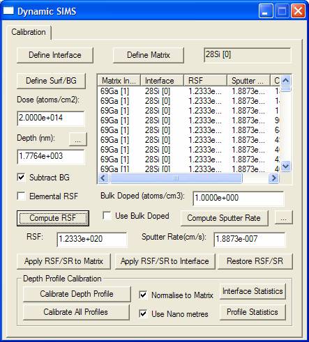
Figure 4: RSF and Sputter Rates are computed from the Dose and Depth, and then entered into the scrolled list.
The new
Experiment Frame contains a VAMAS block for each VAMAS block in the original
file. Within these new VAMAS block, several corresponding variables are defined
which are assigned values for the intensity in counts per second plus the RSF
and sputter-rate used to calibrate the profile. These values can be viewed
using the Crtl PageUp/Crtl PageDown mechanism for stepping through the corresponding
variables in a VAMAS block.
NB: To
compute the elemental RSF from an isotope profile, the tick-box labelled Elemental RSF must be ticked and the
element/transition field for the VAMAS block in use must be set appropriately.
Making Adjustments to the Sputter Rate
A
depth profile prepared for calibration must have an RSF and sputter rate defined
for each matrix within the analysis volume.
If at a later time it is desired to alter the RSF or sputter rate for a
given matrix, the following sequence of steps should be used:
- Select a
cycle from the scrolled-list to identify the matrix for which the RSF or
sputter-rate requires adjusting.
- Press the
pushbutton labelled Restore RSF/SR. The values for the matrix identified by
the chosen cycle are entered into the corresponding text-fields for the RSF and Sputter Rate on the dialog window shown in Figure 3.
- Either the
RSF, the sputter rate or both the RSF and the sputter rate can be
recalculated before again pressing the Apply RSF/SR to Matrix button. The matrix defined by the
selected cycle will be updated with the modified values.
The
same procedure is used to transfer RSF and/or sputter rates from standard
materials to unknown samples. The RSF and sputter rate from a standard sample
are moved from the profile data to the Dynamic SIMS Calibration property page
by first, displaying the data for an element from the standard in the Active
Tile, selecting a cycle in the scrolled-list and then pressing the Restore RSF/SR button. The RSF and
sputter-rate are copied from the selected cycle and entered in to the RSF and Sputter Rate text-fields. Provided the corresponding trace in the
unknown sample is prepared with matrix information and a cycle is selected,
displaying the unknown trace in the Active Tile then pressing the Apply RSF/SR to Matrix button completes
the transfer.
Display of Calibrated Profiles
The
labels for identifying the X and Y axes in a display tile are determined from
the first VAMAS block with respect to the order of selection in the
right-hand-side of the Experiment Frame at the time the VAMAS blocks are
overlaid in the display tile. If a row of VAMAS blocks are selected by clicking
on the experimental-variable value for the row, then the left-most VAMAS block
will determine the axes labels. When a profile is calibrated, in the event that
the left-most VAMAS block in row is an un-calibrated profile, for example a
matrix trace, the data in the un-calibrated profile will be scaled to the range
of the data for all the calibrated profiles in the row and will therefore be
assigned a Y axis label of “Arbitrary Units”. To display an overlay of the
profiles where the Y axis is labelled with respect to a calibrated profile,
namely “Atomic Density”, it is necessary that a calibrated VAMAS block is
selected first. To select VAMAS block in an arbitrary order, left-click the
first VAMAS block, then hold the Ctrl keyboard key down and left click the
other blocks required for the display. The traces are displayed in the Active
Tile by pressing the overlay toolbar button ![]() and
are ordered with respect to the selection sequence.
and
are ordered with respect to the selection sequence.
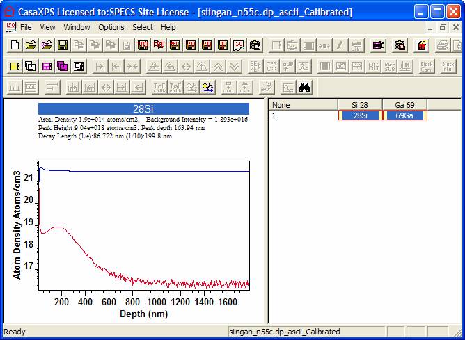
Figure 5: Calibrate Depth Profile