Dynamic SIMS
Calibration of SIMS depth
profiles
SIMS depth
profiles are calibrated from counts per cycle/cycles to atomic density/depth
using Relative Sensitivity Factors (RSF) and sputter rates. Computation of
these conversion factors and subsequent assignment to complex matrix structures
is performed on the Dynamic SIMS dialog window available from the SIMS toolbar![]() . The
SIMS toolbar may be displayed using the View menu on the CasaXPS Main Window.
. The
SIMS toolbar may be displayed using the View menu on the CasaXPS Main Window.
![]()
Figure 1 SIMS toolbar.
Logical Structure of a SIMS Depth Profile within CasaXPS
A depth profile is a collection of VAMAS block all assigned
to the same experimental variable value; typically the experimental variable
will be an index number for a given file of data. There may be more than one
profile per VAMAS file, where each profile will occupy a row as viewed via the
right hand side VAMAS file browser pane. For each VAMAS block within a raw
depth profile, a number of corresponding variables are setup to offer fields
for use in the quantification step. The important fields for quantification are
displayed in the Matrix Index table on the Dynamic SIMS dialog window (Figure
2).
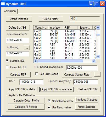
Figure 2: Dynamic SIMS Calibration Dialog Window.
Computation of RSF and
Sputter Rate Values
RSF values
are computed from standard materials using one of three approaches:
- Matrix, dopant
and crater depth.
- Matrix, known bulk doped atomic
density and crater depth
- Interface assignment with
respect to depth and atomic density.
The computation
of the RSF requires the determination of values from the Matrix signal and also
the Implant. To support the determination of these quantities the matrices
within a profile must be identified and a pair of regions defined to specify
the surface zone as well as the appropriate background signal for a given mass.
Defining
the matrix is achieved as follows:
Single matrix materials
- Display the matrix signal for
each profile in the active display tile.
- Press the Define Matrix button
on the Calibration property page on the Dynamic SIMS dialog window. A
pop-up window will inform you that no matrix index is selected and asked
whether the displayed matrix should be applied to all Cycles. Answer by
pressing the Yes button. To avoid the warning message, before pressing the
Define Matrix push button, first select all the table entries by pressing
the header button for the column labelled Matrix Index. If there are any
rows currently selected it will be necessary to de-select these rows
before pressing the header Matrix Index.
If the file
contains more than one depth profile and the matrix for each profile is
overlaid in the active tile, then the operation of defining the matrix for each
depth profile is performed in one go.
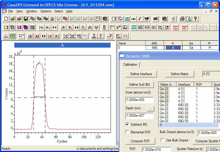
Figure 3
Layered materials
Complex
structure in a material requires the definition of both the matrix material and
also the layer structure. The procedure for defining the matrix and also the a layer is identical except for different buttons are
used to make the assignment.
- Display the signal for one mass
in the active display tile.
- Either using the table or the
mouse (see below), select ranges of cycles within the Matrix Index column
of the table on the Dynamic SIMS dialog window.
- Press the Define Matrix or
Define Interface button (Figure 2 and Figure 3) depending on whether the
matrix or a layer is being assigned. Only those cycles selected in the table
will be assigned to each element within the experiment.
The
matrix/layer structure is used to update the appropriate cycles with the RSF
and sputter rates.
Selecting
rows within the Matrix Index table is achieved using the table together with
the Shift and Control Keys. Alternatively, the selection can be defined using
the active tile and the mouse. When the Shift Key is held down and the left
mouse button is used to drag over the display, the set of cycles corresponding
to those lying between the vertical cursors (Figure 3) will be selected in the
Matrix Index table. This aids the identification of layered structures viewed
via the matrix signal trace. Once a set of layers are so indicated, the
assignment is made by pressing the Define Matrix or Define Interface button.
Defining
the Surface and Background Regions:
- Display any number of VAMAS
blocks in the active display tile.
- Press the Define Surf/BG button
(Figure 2).
Two regions
will appear on each profile; the left most region
indicates the peak and should be adjusted to start just after cycles associated
with any surface spike. The second right-most region defines the background to
the tail of an implant. Both regions can be adjusted using the Quantification
Parameters dialog window when viewing the Regions property page (available from
the Option menu). The left mouse button may be used to drag the start and end
position of these regions whenever the Region property page is active.
Adjustment under mouse control is available when grey vertical lines at either
end of the regions are displayed which appear when the Region property page is
active.
Once the
matrix and regions have been defined, the RSF can be computed by the
appropriate method:
- Either: enter the Implant dose
in Atoms/cm2 and the measured crater depth in nanometres then
press the Compute RSF button and also the Compute Sputter Rate buttons.
Pressing these buttons will result in the corresponding values appearing
in the boxes below the buttons.
- Alternatively, if a bulk doped
standard is in use, tick the box labelled Use Bulk Doped and enter the known atom density into the above
data input field. Both the implant and matrix require regions when a bulk
doped standard is used to compute the RSF.
- The third method for computing
the RSF is via a known implant depth and atom density. The button to the
right of the Depth field, namely,
 results in a dialog window in which a depth and/or a peak intensity can be
entered (Figure 4). The position of the implant is defined using the
Matrix Index table by making a single selection in that table. The
appropriate cycle can be identified by left-clicking on the peak in the
left-hand-side active tile. The Matrix Index table scrolls to show the
cycle corresponding to the mouse selection and the table entry is
therefore offered for selection prior to invoking the Define Depth by
Cycle dialog window in Figure 4. If the correct depth and corresponding
atoms per cc are entered, the Calc RSF tick box is ticked and the OK button
is pressed, the RSF, Depth and Sputter Rate fields will be updated.
results in a dialog window in which a depth and/or a peak intensity can be
entered (Figure 4). The position of the implant is defined using the
Matrix Index table by making a single selection in that table. The
appropriate cycle can be identified by left-clicking on the peak in the
left-hand-side active tile. The Matrix Index table scrolls to show the
cycle corresponding to the mouse selection and the table entry is
therefore offered for selection prior to invoking the Define Depth by
Cycle dialog window in Figure 4. If the correct depth and corresponding
atoms per cc are entered, the Calc RSF tick box is ticked and the OK button
is pressed, the RSF, Depth and Sputter Rate fields will be updated.
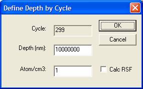
Figure 4
Once an RSF is computed and the appropriate Sputter Rate
entered for an implant in a given matrix, the profile can be update with these
values: select a cycle from the Matrix Index table with the appropriate the
matrix entry and press either the ![]() button or the
button or the ![]() button. Each cycle within the profile with the
same entry as the selected matrix index will be updated with both the Sputter
Rate and the RSF. If the material is a multilayer structure the procedure
should be repeated for each layer, where the RSF and Sputter Rates are first
determined from a standard profile. An RSF/Sputter Rate pair can be extracted
from another profile by first displaying the profile, making a selection in the
Matrix Index table and pressing the
button. Each cycle within the profile with the
same entry as the selected matrix index will be updated with both the Sputter
Rate and the RSF. If the material is a multilayer structure the procedure
should be repeated for each layer, where the RSF and Sputter Rates are first
determined from a standard profile. An RSF/Sputter Rate pair can be extracted
from another profile by first displaying the profile, making a selection in the
Matrix Index table and pressing the ![]() button. The RSF/Sputter Rate from the
indicated matrix index will be entered into the fields on the dialog window,
thus allowing the unknown to be subsequently displayed and these restored values
from the standard used to update the unknown profile. Note, the Dose and depth
for single matrix material are computed when the Apply to Selected Matrix button is pressed.
button. The RSF/Sputter Rate from the
indicated matrix index will be entered into the fields on the dialog window,
thus allowing the unknown to be subsequently displayed and these restored values
from the standard used to update the unknown profile. Note, the Dose and depth
for single matrix material are computed when the Apply to Selected Matrix button is pressed.
Once RSF and Sputter Rates have been assigned to each depth profile, the data are calibrated by pressing the Calibrate Depth Profile button. If multiple profiles are prepared and overlaid in the active tile, pressing the Calibrate All Profiles button results in each profile, so selected, being calibrated and entered into a single Experiment Frame. The depth scale units must be selected prior to calibration using the tick box Use Nanometres.
Note: If normalization to the matrix is not requires, it is necessary to compute the RSF with the same selection of the Normalize tick box.
Depth Profile Statistics: Areal Density and Decay Length
Areal Density and Decay Length are computed as part of the Depth Profile Statistics. The procedure for calculating these statistics requires a pair of cursors to be defined on the displayed profile in the active tile. The aim is to mark the region over which the profile peak appears. To mark the cursors on the profile: hold the Shift Key down and drag a box starting from the left of the peak and ending at the right-hand end with the mouse positioned at the intensity of the background. On pressing the Profile Statistics button (Figure 2) a dialog window appears showing the current text in the VAMAS block comment plus a set of lines offering the new calculated profile statistics. If it is desired to include these new lines in the VAMAS block comment, then the OK button should be pressed, otherwise the Cancel button will exit without altering the VAMAS block comment. Note, the text in the VAMAS block comment can be edited within this window leaving only the information so required.
Maintaining Standards Library Files
Once standards have been prepared and RSF/Sputter Rates
computed, these depth profiles can be moved to other files containing profiles
from standards. The toolbar buttons ![]() allow VAMAS blocks to be copied into an
existing file and also delete from a file. Once a number of standard material
profiles are located in a single file, the
allow VAMAS blocks to be copied into an
existing file and also delete from a file. Once a number of standard material
profiles are located in a single file, the ![]() button offers a means of searching the strings
within a VAMAS block comment and those matched are both selected in the
right-hand side of the Experiment Frame and are also displayed in the scrolled
list of display tiles. VAMAS block comments can be edited using the
button offers a means of searching the strings
within a VAMAS block comment and those matched are both selected in the
right-hand side of the Experiment Frame and are also displayed in the scrolled
list of display tiles. VAMAS block comments can be edited using the ![]() toolbar button.
toolbar button.
A Multi-Layer Example
In this example, the desired result is a plot of atomic density verses depth for Mg. To achieve this end and owing to the layered structure, four masses were monitored, where two labeled 69G and A define the layer structure while the trace labeled Ga represents a constant matrix signal, to which the Mg signal is normalized.
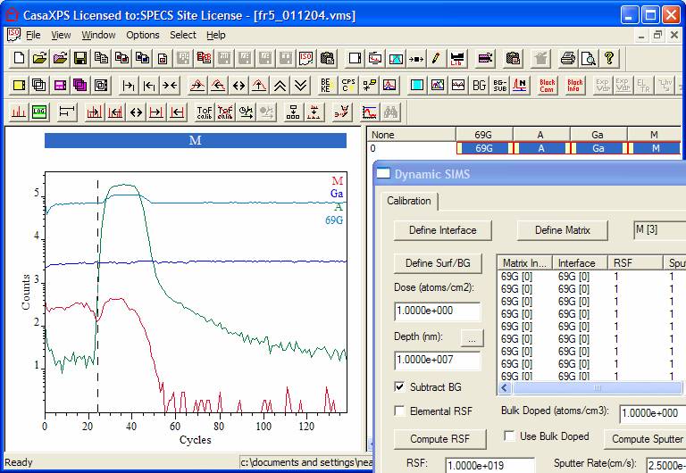
Figure 5
Step 1: Define the Matrix
Display the matrix, namely, Ga in
the Active Tile. The block id plus the VAMAS Block index for the trace will
appear on the Dynamic SIMS dialog window (indicated within the red box). Select
all the cycles under the Matrix Index column in the table on the Dynamic SIMS
dialog window and press the Define Matrix button (also indicated within the red
box). The selected entries under the Matrix Index column will change to say Ga [2] and thereby showing the matrix is defined.
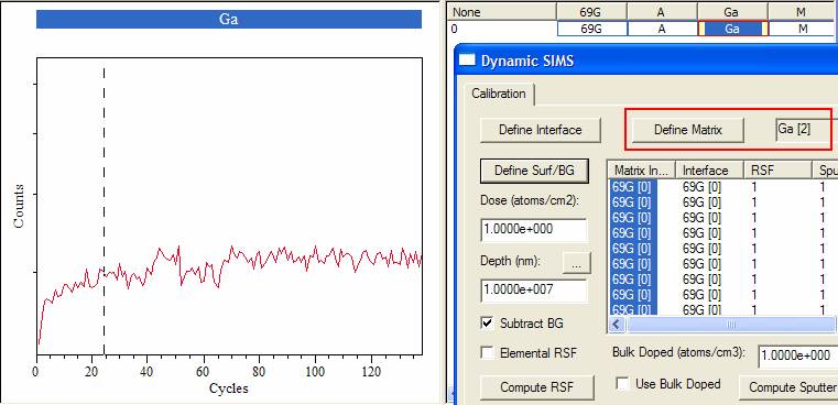
Figure 6
Step 2: Define the Layer Structure
The material is GaN : AlGaN : GaN
in structure (Dr Shadi Shahedipour,
Mark the AlGaN layer by holding the Shift-Key down and then dragging a box from the left to the right of the AlGaN peak. The result of such an action is shown in Figure 3. All the cycles within the table on the Dynamic SIMS dialog window between the vertical cursors shown on Figure 3 are selected by the mouse action and so pressing the Define Interface button on the same property page will cause the Interface column in the table to be updated.
Step 3: Enter RSF and Sputter Rate Values
In this example the RSF and Sputter Rate for the two layers are assumed to be known. All that is required is to add sputter rates and RSF for each of the three layers; the values are entered on the Dynamic SIMS property page in Figure 2, a given matrix or interface cycle is selected and the table entries corresponding matrix or interface updated by pressing Apply RSF/SR to Matrix or Apply RSF/SR to Interface, as desired. In this example, two RSF and SR pairs are entered corresponding to the GaN and AlGaN layers. Since the matrix does not define the layer structure, the assignments are made by using the Apply RSF/SR to Interface button. After displaying the Mg trace in the Active Tile the RSF/SR can be entered. Firstly, both the GaN layers are assigned by selecting one cycle for which the interface column contains 69G [0], entering the appropriate RSF/SR and pressing the Apply RSF/SR to Interface button. Each cycle previously designated as part of the 69G [0] layer will receive the RSF/SR pair. Similarly, the AlGaN RSF/SR values are entered in the text-fields, one cycle with an Interface column of A [1] selected and the Apply RSF/SR to Interface button pressed a second time. Again, each cycle designated as Interface A [1] will receive the RSF/SR pair. (Figure 7)
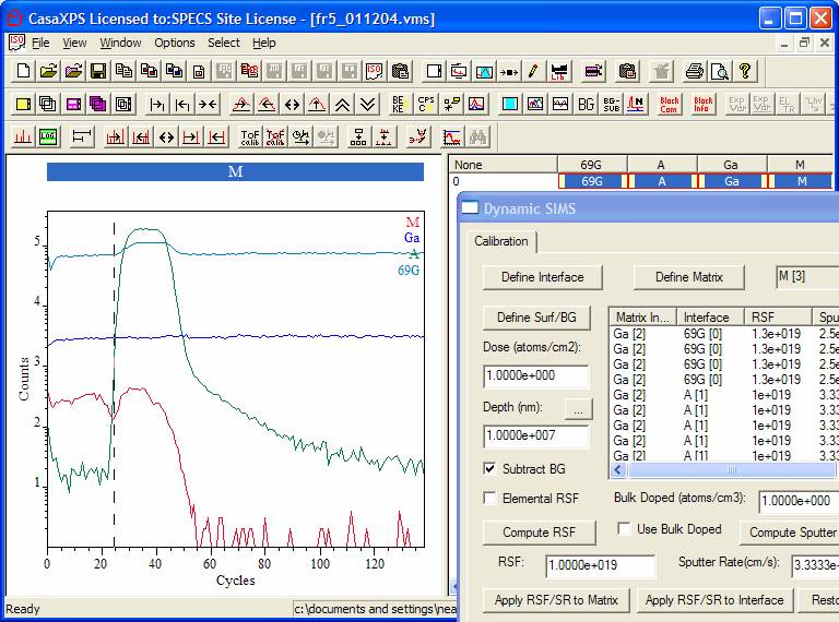
Figure 7
Step 4: Calibrate Mg Profile
Calibration is performed by displaying the profile in the Active Tile and pressing the Calibrate Depth Profile button in Figure 2.
In this example, the only mass for which RSF/SR pairs are entered is Mg. The SR are automatically assigned to all masses, however the RSF values for masses other than Mg remain set equal to unity. A consequence of leaving an RSF equal to unity is that on Calibration to atomic density and depth, masses for which the RSF is equal to unity will be scaled to the atomic density range of any properly calibrated masses. This allows an overlay with respect to the calibrated traces, without requiring the RSF for all masses to be assigned prior to calibration. Counts per second traces are available in the calibrated Experiment Frame as the second corresponding variable (Ctrl PageUp/Crtl Page Down).
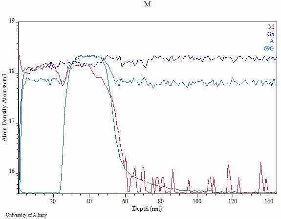
Figure 8: Calibrated Mg profile with scaled A/Ga/69G data.
An Example of Computing an RSF
The profile in Figure 9 was obtained from GaN undoped epi growth ion implanted with 24Mg at a dose of 1.0e15 atoms per cm2. The depth at the peak of the Mg counts is 77 nm. Computation of an appropriate RSF is performed as follows:
Step 1: Define the Matrix
Display the Ga2 matrix profile in the Active Tile, press the
header button labeled Matrix Index in the table to select all cycles and press
the Define Matrix push button on the Dynamic SIMS dialog window. The table on
the same dialog window will update to show that the Matrix index for each cycle
is now assigned to the Ga2 profile.
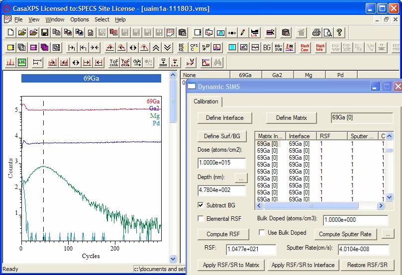
Figure 9
Step 2: Define the Surface Layers and also the Background for the Mg Profile
Display the Mg profile in the Active Tile and press the button labeled Define Surf/BG. Two regions are created on the Mg profile. The left-most end of the left-most region defines the surface layers, while the background to the right-most of the two regions estimates the background to the Mg signal.
Step 3: Define the Depth Scale
In this example, the depth scale is defined to be 77nm at
the maximum signal for the Mg profile. Using the left-mouse button, click on
the profile to indicate the position of the Mg maximum values. The table
entries on the Dynamic SIMS dialog window will scroll so that the cycle,
corresponding to the position of the vertical cursor, is located at the top of
the visible portion of the list. Select the entry at the top of the visible
portion and press the button next to the Dept (nm): label (Figure 10). A dialog
window appears in which the selected cycle index in already entered and a
text-field for the Depth (nm) corresponding to the indicated cycle can be
input. On pressing the OK button, the Dynamic SIMS dialog window in updated
with the Depth computed from the Define
Depth by Cycle dialog window values.
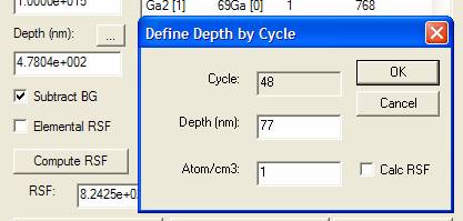
Figure 10
Step 4: Enter the Dose and Compute the RSF
Enter the dose in atoms per cm2 on the Dynamic SIMS dialog window and press the button labeled Compute RSF. If the elemental RSF is required, the tick-box just above the Compute RSF button should be ticked (Figure 10).
Step 5: Calibrate the Mg Profile
Once the RSF is computed and the sputter rate updated, the values for each cycle corresponding to the Mg profile (currently displayed in the Active Tile) must be updated. In this example, the assignment for the matrix is sufficient to target the cycles for which RSF and sputter rates must be applied. Simply select any cycle using the Matrix Index column in the table and press the Apply RSF/SR to Matrix button. Since all the cycles are defined to have the same matrix, the table for the Mg profile will contain values for the RSF and sputter rate throughout. To calibrate the profile, press the button labeled Calibrate Profile.
The calibrated profile for Mg is shown in Figure 11. Note
that the Profile Statistics button (Figure 2) has been used to create a VAMAS
block comment showing the Areal Density and Decay
Length for the Mg profile. Also note how the profiles for which no RSF is
specified are scaled to allow their visualization within the same scale as the
calibrated Mg profile.
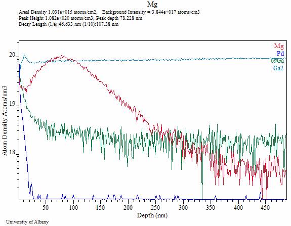
Figure 11