For further information about XPS/AES data processing please visit: http://www.casaxps.com/

Uncertainties in Peak Parameters Based upon Monte Carlo Simulation

Optimization routines are completely deterministic, in that, for the same set of parameters, used in the same functional forms, applied to the same set of data, with the same initial and final conditions will result in the same set of parameters on termination. Vary any of the above conditions and the result from the optimization routine will change in some respect. One method for assessing the uncertainty in the parameters for a peak model is to vary these optimization conditions by repeating an experiment on, what are hoped to be, identical samples. Then for each set of data apply the same optimization routine to the same synthetic model and so determine a distribution for the set of parameters used to quantify a sample. Such a procedure will vary almost every aspect of the measurement process and so result in a distribution for the parameters that truly represent the nature of the experiment.

The basis for such an approach as described above lies in the assumption that there exists a set of parameters (only known to nature) that does not depend on any optimization routine nor any other errors introduced into the measurement process, and these true values will lie inside the region of the N-dimensional parameter space defined by the set of outcomes to this sequence of experiments. Obviously, if the synthetic model does not describe a set of parameters in tune with nature, the results may be in more doubt than the measured distribution might suggest. However, given that all is well then the task is to offer a means of understanding the uncertainties in the peak parameters within the context of these parameter distributions.

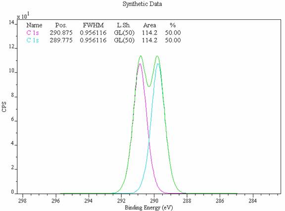
Peak identification in XPS spectra represents a challenge since synthetic models more often than not involve overlapping line-shapes (Figure 1), the consequence of which is correlated optimization parameters. That is to say, if a single data envelope results from two overlapping peaks and if one of these underlying peaks is reduced in intensity then in order to describe the same data envelope the other must increase in intensity. Adjustments to peak parameters of this nature are inherent to any optimization procedure and the choice between the possible combinations of these peak intensities is made based upon a chi-square or root-mean-square metric. The problem is therefore to identify the point at which these goodness-of-fit metrics fail to produce results that can be believed, and provide some means of illustrating the degree of uncertainty.

Given a distribution for each of the parameters, the best way to describe the nature of the uncertainties is to offer an error matrix as well as a tabulated form for the distributions. The error matrix provides numerical values from which the degree of correlation can be assessed while scatter plots taken from some subset of these distributions allows visual inspection for the same information. Ideally a single number for each parameter would provide the simplest means of stating the uncertainties, but as the old adage goes “To every complex problem there is a simple solution that is wrong”, and so it is for correlated parameters. The unfortunate fact is that if the peaks weren’t correlated then synthetic models would be unnecessary.

Monte Carlo Data Sets

Repeating an experiment many times is not always practical and for most XPS spectra peak models are developed based upon a single acquisition sequence. Estimates for uncertainties in the peak parameters must be made using assumptions about the noise typical of XPS spectra. The essence of Monte Carlo methods for estimating uncertainties is to take a data set, remove the noise from the data, then repeatedly add noise to the synthesized data to generate a set of simulated experimental results and apply the set of operations to that artificial data. The results represent a distribution for each of the parameters from which an error matrix and tabulated parameter distributions can be extracted.

Error Matrix

The result of a Monte Carlo simulation for a peak fit takes the form of m optimization parameters from each of the n simulated data sets. An error matrix derived from these parameter distributions is defined to be an m x m matrix as follows:

.

Where the x_sik are parameter values calculated for each of the simulation steps and each distribution is centered with respect to the mean rather than the initial parameter value.

The standard error in each parameter is given by

and the correlation between parameters i and j is given by

.

An alternative method for estimating uncertainties in the peak parameters is to quote the inverse of the Hessian matrix used in the Marquardt Levenberg optimization routine. So the question is, why bother with Monte Carlo simulation when this very information desired is offered by the optimization procedure itself. The answer comes in two forms. Firstly, the error matrix derived from Monte Carlo is not limited to the problem of just fitting the peaks. The simulation procedure can also take account of the background as well as the peaks, and so determine a global error matrix for the calculation rather than one that focuses on the stability of the peak parameters alone. Secondly, the Hessian matrix has a tendency to be near singular when the Marquardt algorithm terminates. Indeed the optimization routine follow a sequence of steps that switch between a direct solution of the Hessian matrix and a solution of a regularized form of the matrix. The regularization step occurs when the direct Hessian inversion fails to produce an improvement in the fitting parameters and a common reason for this to occur is that the Hessian is ill conditioned. Under these circumstances the covariance matrix derived from the Hessian should not be trusted.

Figure 1: Simulated PVC C 1s Data Envelope.

Monte Carlo: A Simple Example

The best way to introduce the ideas behind Monte Carlo methods and how the results can be interpreted is to look at a simple example.

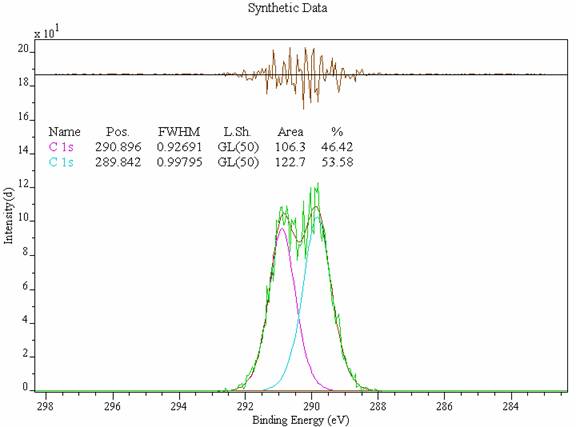
Consider the data envelope in Figure 1. The spectrum is a synthetic envelope created from two GL (50) line-shapes without any background and where the peaks are separated by an energy gap consistent with C 1s lines in a PVC spectrum. In the absence of noise and experimental error the optimization routine always returns the peak parameters tabulated on the spectrum in Figure 1. The next step in the simulation is to introduce noise onto the data envelope that is consistent with noise found in experimental XPS spectra, i.e. variations about the channel intensity of magnitude related to the square root of the counts. Figure 2 shows the data envelope from Figure 1 after noise has been added and the peak parameters refitted.

Figure 2: Simulated C 1s data where noise has been introduced to the system.

This procedure yields the first set of simulation results. If repeated many times, the output is six distributions, one for each of the peak parameters involved and these can be used to assess the influence of experimental noise on these quantities. Note that this differs in some respects from adopting a purely experimentally determined parameter distribution. The initial stating point for the peak parameters will not be identical for an experimental data set since the experimental data may be subject to sample charging, and any errors in the measurement procedure that can not simply be described by the random nature of the counting system will be omitted. A Monte Carlo simulated data set only tests the stability of a model with respect random noise and therefore may neglect other factors present in an experimental data set.

Table 1: Error Matrix for the C 1s spectrum in Figure 1.

	1:Area	1:Pos.	1:FWHM	2:Area	2:Pos.	2:FWHM
1:Area	39.230	0.122	0.196	-31.512	0.128	-0.186
1:Pos.	0.122	0.001	0.001	-0.120	0.000	-0.001
1:FWHM	0.196	0.001	0.002	-0.185	0.001	-0.001
2:Area	-31.512	-0.120	-0.185	38.330	-0.125	0.202
2:Pos.	0.128	0.000	0.001	-0.125	0.001	-0.001
2:FWHM	-0.186	-0.001	-0.001	0.202	-0.001	0.002

Table 1 is the error matrix that results from a Monte Carlo simulation for the spectrum and synthetic model in Figure 1. If viewed as uncorrelated error distributions (which is certainly not true) then one standard deviation in each of the parameters is given by the square root of the diagonal elements in the matrix. It may be seen that the areas of the two peaks are anti-correlated, where the quantity –31.512 / Ö(39.230 x 38.330) characterizes the degree of interaction between the two parameters. The minus sign indicates the parameters are anti-correlated. A scatter plot constructed from the two distributions for the peak areas is shown in Figure 3, where the anti-correlation is obvious from the bias in the scatter along a direction 135° to the positive x axis. An alternative scatter plot (Figure 4) for the area and FWHM parameters taken from peak C 1s 1 (Figure 1) shows that these two parameters exhibit positive correlation.

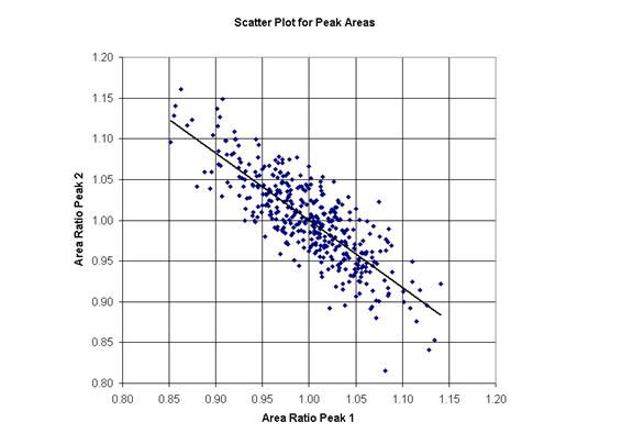
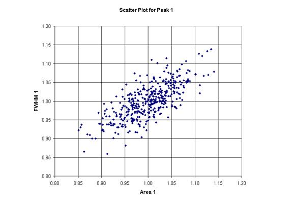
The uncertainty for correlated parameters can be estimated from plots such as those shown in Figure 3 and Figure 4. By projecting horizontal or vertical lines onto the parameter axes in such a way that the appropriate number of points lie between the projection lines for a given confidence limit, the uncertainty for a parameter can be assessed in the context of others. Again, the uncertainty for a parameter should be viewed in the context of all other correlated distributions, and yet the ellipsoid in 6-dimensional parameter space is difficult to quantify; the procedure based on scatter plots should be seen as merely a step in the right direction rather than arriving at the ultimate destination. In the case of the peak area shown in both Figure 3 and Figure4, the estimate taken from the diagonal element of the error matrix would seem to be reasonable. Both scatter plots show that about 65% of the points lie inside projection lines positioned at about 0.95 and 1.05. This interval represents about ±5% of 114.2 CPSeV (see Figure 1) and is not too different from the uncertainty taken from the error matrix ±6.2 CSPeV.

Figure 3: Scatter plot showing the anti-correlation between the peak area parameter distributions.

Figure 4: Scatter plot between Area and FWHM parameters for Peak C 1s 1 in Figure 1

All the parameter distributions are reported relative to the initial parameters used to define the data envelope. As a result the relative parameter distributions may not be symmetrical about the initial value and asymmetric confidence intervals are possible. Note that the error matrix is calculated from the distributions centered on the mean parameter value for the distribution, not the initial values.

One of the real advantages of using Monte Carlo error analysis is that it highlights when a quantification parameter is poorly determined by the combination of model and optimization procedure. It also allows the influence of constraints within a model to be evaluated. Adding information about chemical shifts, relative peaks widths and/or peak areas can alter the manner in which noise adjusts the parameters from their initial value. Monte Carlo derived scatter plots can often help to understand how rigid models based upon chemical knowledge can reduce the range of outcomes for a given set of parameters.